Diatoms are one of the most abundant biological microfossils in sediment cores and on smear slides. Diatoms are one group of microscopic algae and characterized by their golden-brown pigmentation and having a cell wall made of biologically produced glass or biogenic opaline silica. Because they are made of opaline silica, diatom cell walls are fairly resistant to breakage and dissolution and can form up to 60% of the dry weight in some lake cores (Edlund et al. 2000). The cell wall in a living diatom is put together like a Petri dish; the two halves are called valves with one valve slightly larger and overlapping the other valve. There are a few other parts in the cell wall, primarily hoop or band-like structures called girdle bands that form the overlap between the two valves. Collectively, the siliceous parts surrounding a single cell are termed the frustule. Size, shape, and ornamentation on the valves distinguish the more than 40,000 diatom species in the world. For detailed diatom analysis, sediments are specially prepared using peroxide or strong acids to digest the cell contents; the "cleaned" cell walls are mounted on microscope slides using specialized mountants that optimize resolution of valve ornamentation for species-level identification. More detailed information on diatom preparation and species identification can be found here.
But back to smear slides…you'll find diatoms in your smear slides as single valves, single cells, or many species form characteristic colonies of filaments, bands, zig-zags, or star shapes. Diatoms may be empty, filled with an air bubble, or can even have cell contents remaining (many species of diatoms get buried alive in the sediments as resting cells and can be rejuvenated to grow again even after decades of burial; Sicko-Goad et al. 1989. Scan around your slide at 200-400x (20x or 40x objective) to see how abundant diatoms are in your material. Don't be overwhelmed by their many shapes and forms. Are there lots of different forms or just a few? What kind of shapes do you see: circles, barrel shapes lined up in filaments, banded colonies that look like fences, big ones and little ones, or just lots of funky shapes. There are expert diatomists out there that can help if you want to do a detailed analysis of the diatoms, but learning just a little bit about the diatom flora in your core using the below tutorials can quickly and easily provide some of your first and best paleoenvironmental information. Let's take a look at some simple qualitative and quantitative measures that can be made from smear slides related to abundance, preservation, and diatom ecology.
Diatom abundance
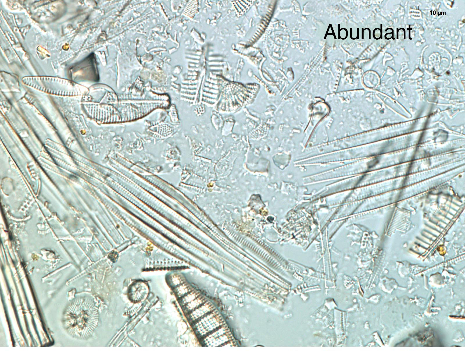
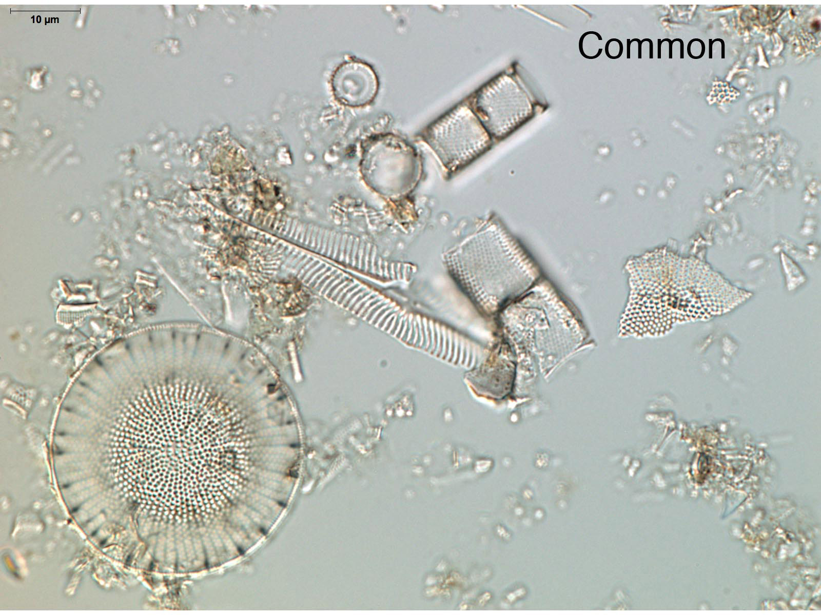
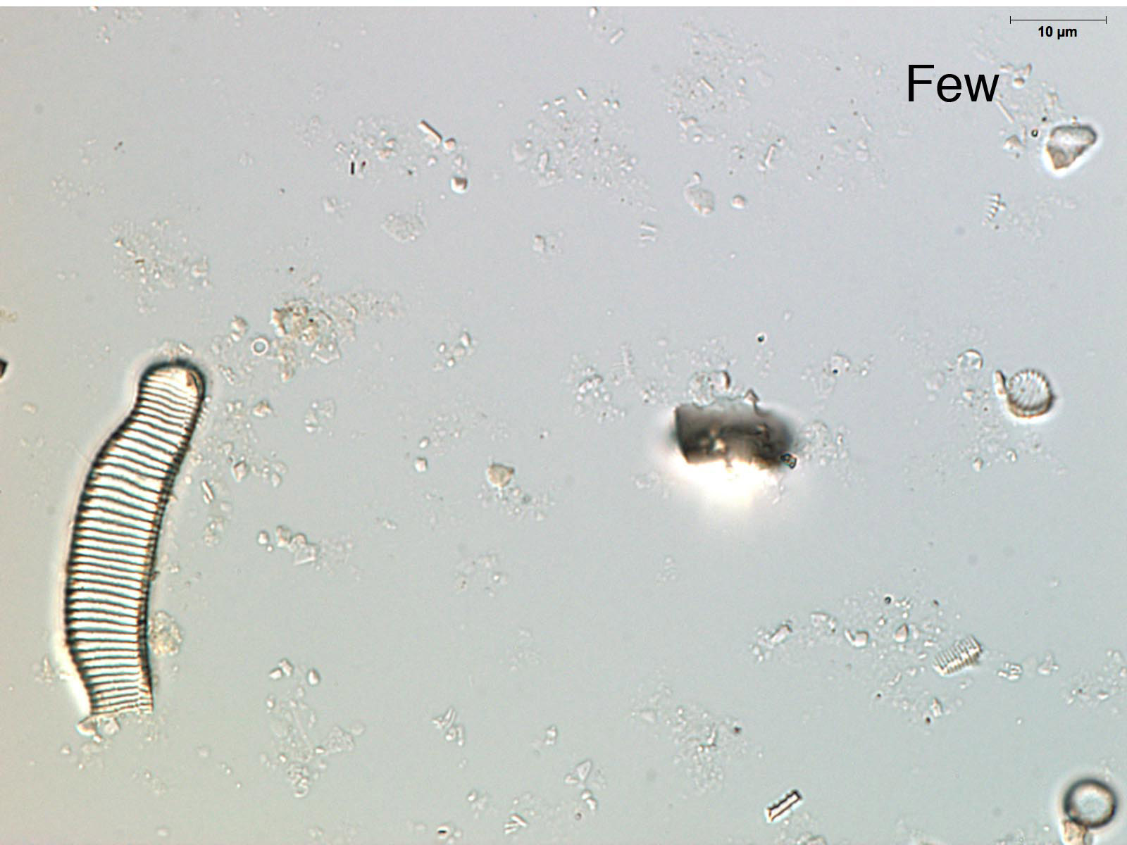
The quantity of diatoms in sediments varies considerably due to the lake's paleoecology, depositional environment, and preservation. Noting the quantity of diatoms in a smear slide can help focus future analyses, show general shifts in lake productivity (e.g., eutrophication events), and identify changes in the depositional environment (e.g., turbidites). If you have carefully made your smear slides using similar amounts of material for each slide, the relative abundance of diatoms can be determined by simple comparison. Look at a few of your slides under 200-400x magnification. The abundance of diatoms present in a smear slide can be reported using a simple relative scale as abundant, common, few, or absent.
Diatom preservation
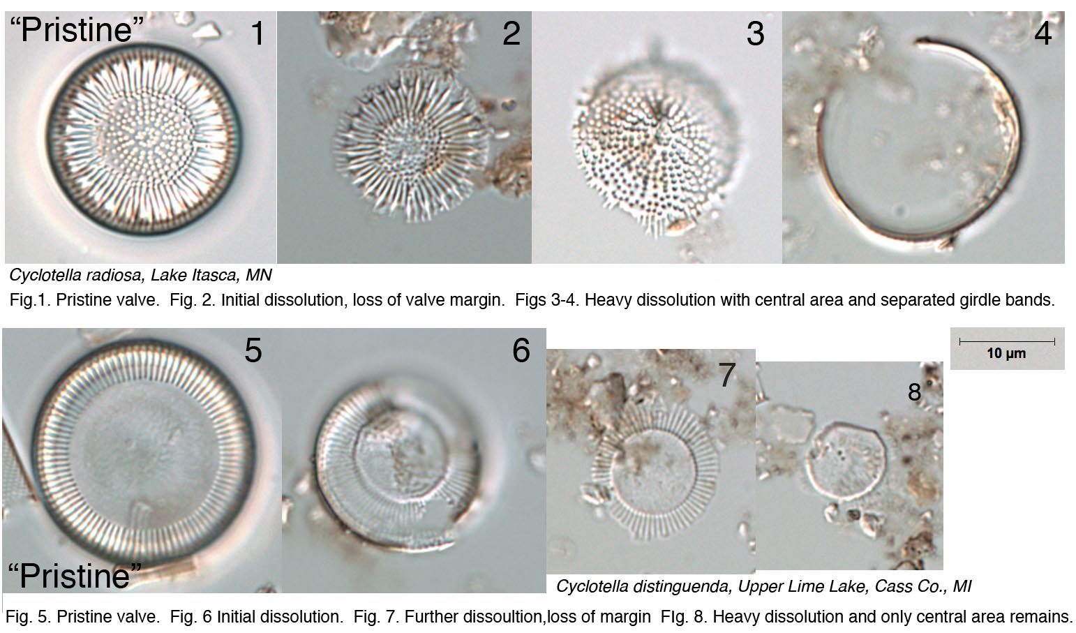
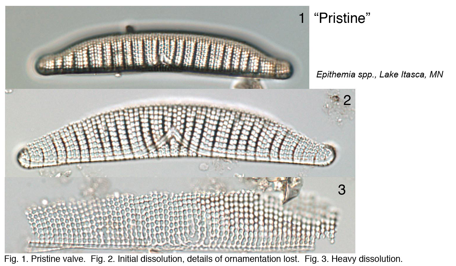
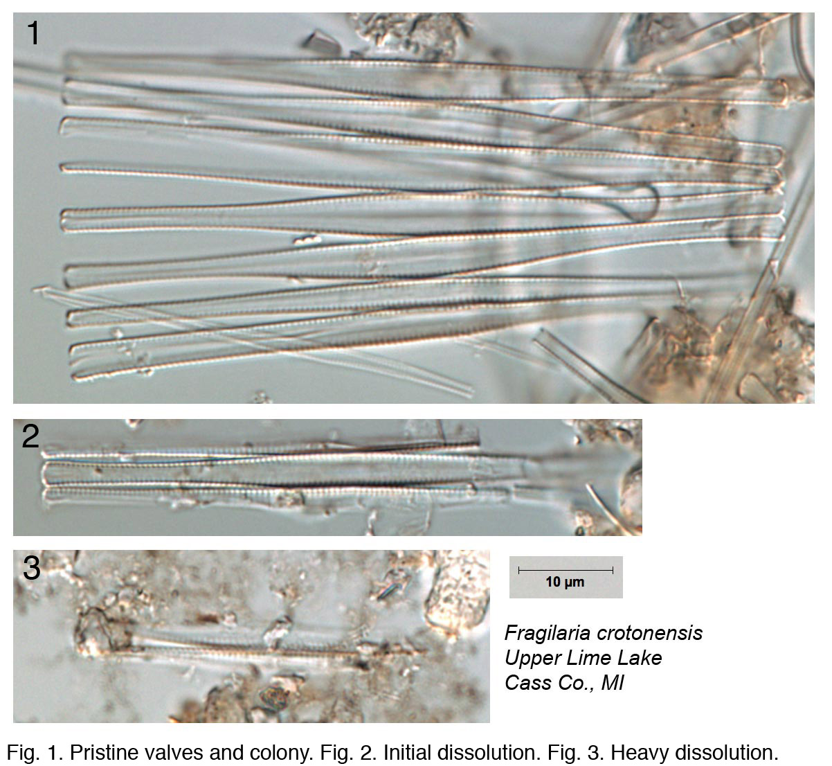
The condition of diatom microfossils in a smear slide is a reflection of the depositional environment and will determine their suitability and usefulness as environmental indicators. Several environmental conditions enhance the dissolution of diatoms: breakage, salinity, alkalinity, and silica-poor environments. Diatom valves are composed of biogenic opaline silica and each valve has areas where silica is deposited more thickly (e.g., central areas, raphe ribs) as well as areas with patterns of ornamentation comprising holes (areolae, pore fields) and lines (striae). The dissolution of diatoms generally follows a pattern where highly ornamented or thin areas are lost first, followed by sequential loss depending on silica thickness, until only the most heavily silicified areas of the diatom remain. Diatom species are also differentially susceptible to dissolution. A simple metric (% pristine) based on the condition of diatom microfossils in smear slides can be used to summarize the level of dissolution in your samples.
Examples:
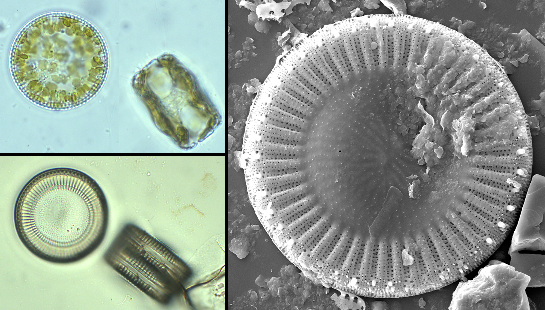
Cyclotella species
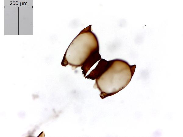
Epithemia species
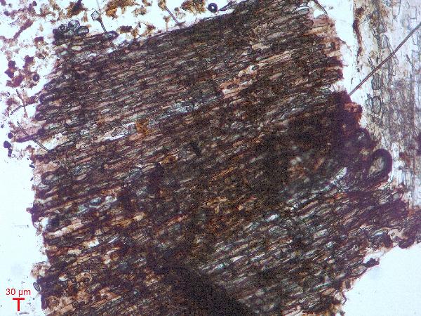
Fragilaria species
Ryves et al. (2001, 2009) discussed issues surrounding diatom dissolution in sediment cores, proposed several indices to describe dissolution artefacts, and offered insights into how dissolution might affect interpretation of paleorecords.
Diatom ecology – plankton:benthic ratio
Diatoms can be ecologically separated in two broad categories: planktonic species that live in the water column and benthic species that live in the sediments or attached to rock, plant, or other substrates. A ratio called P:B or the planktonic:benthic ratio provides a simple metric of possible changes in the paleoenviroment based on lake level change or nutrients. The ratio is often expressed as a percentage, i.e. a P:B ratio of 1.0 would equal 50% percent planktonic species. Depending on lake morphometry lake level changes can result in dramatic shifts in the proportion of open water and littoral zone habitat (Wolin and Stone 2010). Sediments preserve a temporal and spatial integration of a lake's diatom communities so periods with greater littoral zone extent will generally have great benthic diatom numbers. The other major factor that drives changes in P:B is lake eutrophication. Nutrient addition to lakes often results in proportionally greater planktonic diatom growth and higher P:B ratios (Edlund et al. 2009).
Calculating the P:B ratio for your smear slides requires two steps. First let's learn how to recognize planktonic vs benthic diatom, and try out our skills. Then we'll discuss how many fields might be appropriate to count to get a representative value for your smear slide.
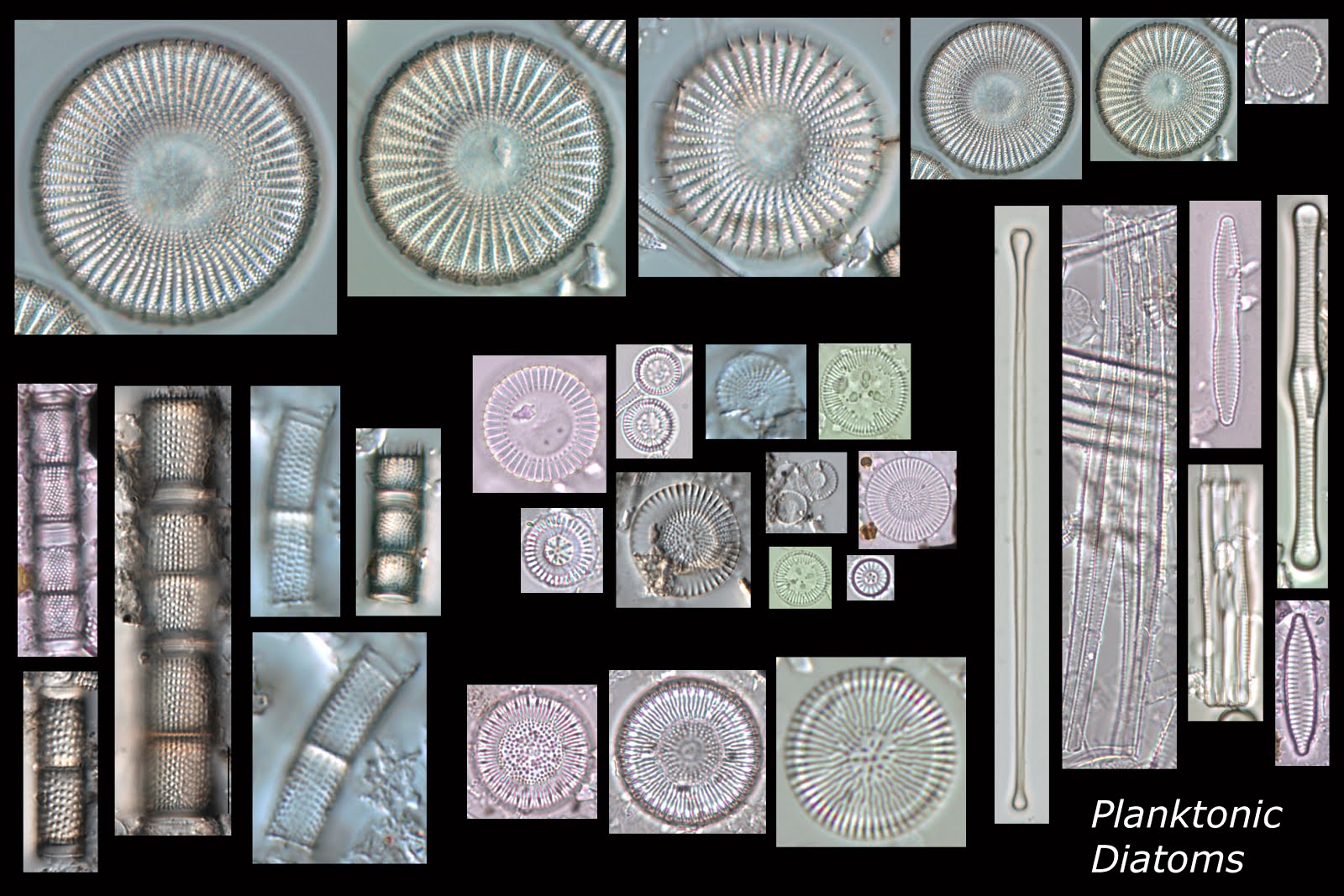
Diatoms come in all shapes and sizes. Planktonic species generally have five common shapes: circular, barrel-shaped in filaments, band shaped colonies, star or zig-zag colonies, or long thin species. Here's a montage of many planktonic forms:
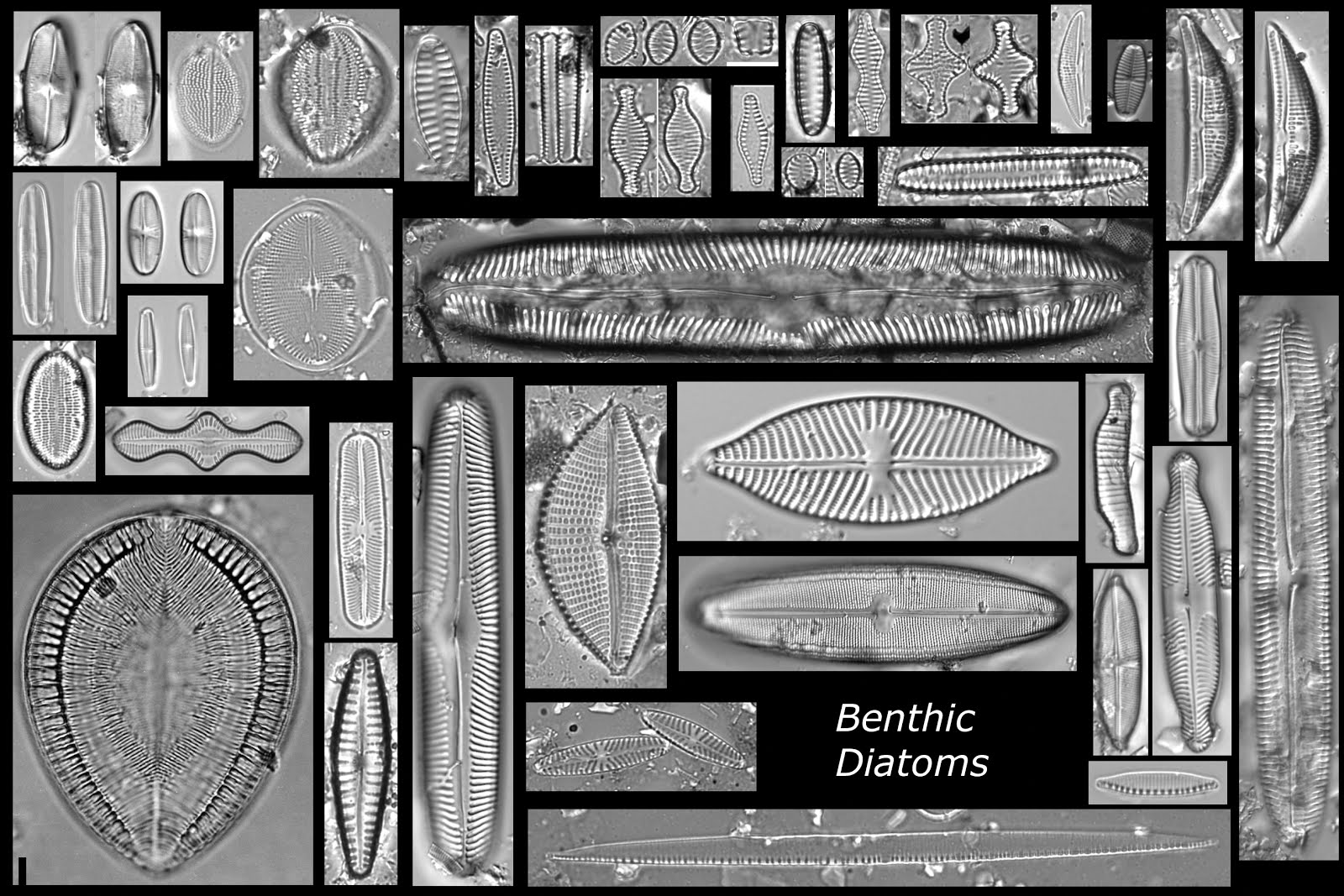
Benthic diatoms also vary in shape, but few will be round, rather most have a shape that is symmetric along a line and more similar to the outline of a boat (oval or elliptic), or shaped like the moon (lunate) or a club, and all may have variously shaped ends. Here's a montage of many different benthic species:
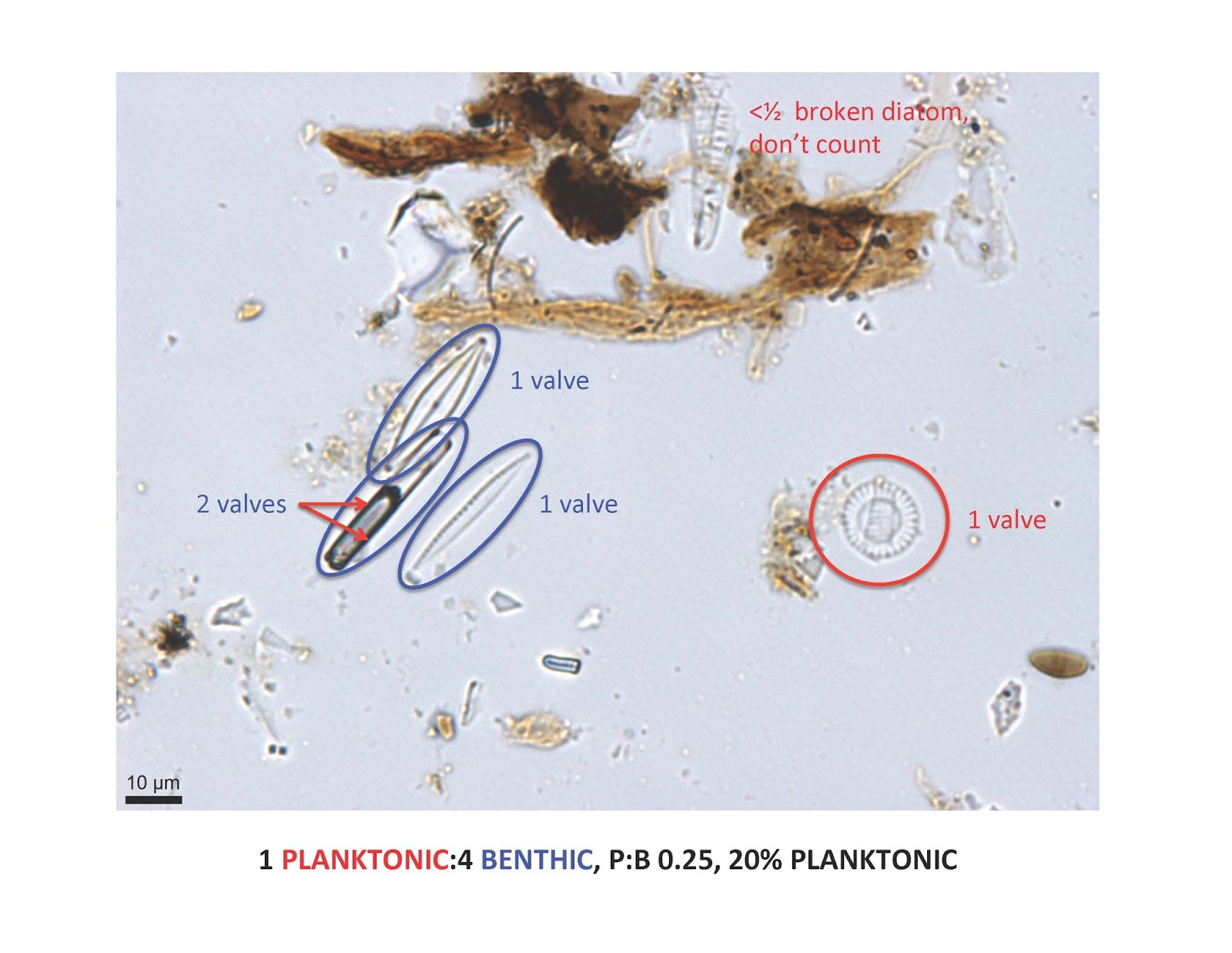
Let's look at some pictures from smear slides and see how easy it is to calculate a P:B ratio. This is an image from a eutrophic lake in Minnesota. Can you refer to the montage of planktonic and benthic diatoms and then count how many diatom valves you see from each category? Remember that each cell of a diatom has two valves—sometimes they remain together in a cell, other times they get dissociated. In real life, you may need to focus up and down a bit to figure out if both valves are there (Hint: an air bubble in the diatom usually means there are two valves). Here's an easy one:
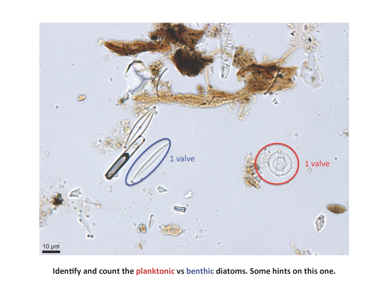
Did you get 1 planktonic and 4 benthic for a 1:4 or 0.25 P:B or 20% planktonic species? Note one of the diatoms has both valves and it's laying on its side, and we usually don't count a broken valve with less than ½ a diatom.
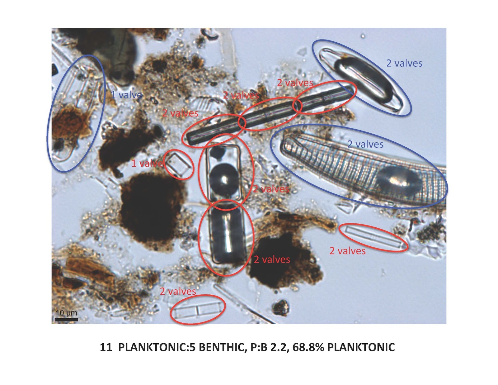
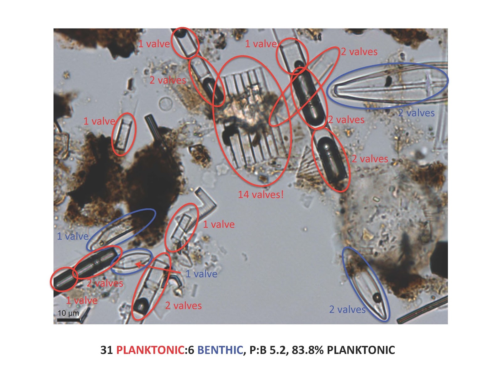
Heres another image, a little tougher:
Heres another image, a little tougher:
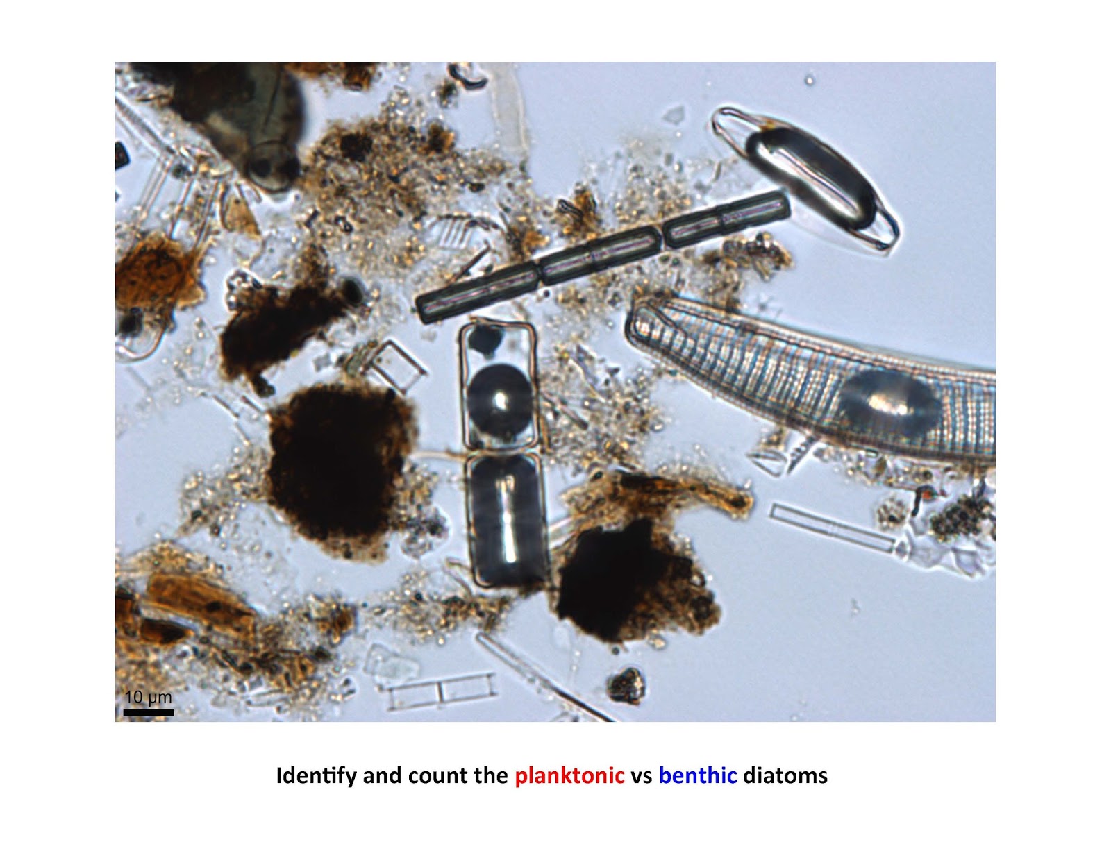
Did you find all 16 diatom valves on that last one. Note that when there is an air bubble in the diatom, usually both valves are present.
You can see that the density of diatoms and the ease of counting varies among slides. To generate good P:B data you will need to count multiple fields on a slide until your P:B number converge on a value. It is easy to just enter your data into a spreadsheet as you count each random field on your smear slide. Keep a running estimate of your P:B scores and consider your count complete once you converge on a stable value. Typically diatomists count between 400 and 600 diatoms to get these values; you may be able to count fewer.
Diatom ecology – diatom:cyst ratio
Another important and easy set of data to recover from smear slides is the ratio of diatom valves to chrysophycean cysts, or the cyst:frustule ratio, which is usally reported as the percentage of cysts to the total of cysts plus frustules. The chrysophytes and synurophytes are two groups of golden-brown microalgae that have incorporated siliceous structures into their vegetative cells (as a coat of siliceous scales and spines) and life histories. As part of their life history, many species produce siliceous resting cysts that are variously referred to as chrysophycean cysts, statocysts, statospores, or hypnospores. Both the cell coat components (scales and spines; often analyzed in detail to determine pH changes; Zeeb and Smol 2001) and cysts can be found abundantly in sediment cores and smear slides.
The rato of cysts:diatom valves was first recognized by Smol (1985) as a way to distinguish the relative importance of each group in a lake's sediment record. The ratio was later shown to be responsive to several environmental drivers and gradients. For example, in temperate lakes lower numbers of chrysophyte cysts relative to diatoms is a classic sign of eutrophication (Smol 1985). In arctic lakes, the ratio is responsive to past extent of ice cover, with higher values of cysts:frustule during periods of greater ice cover (reviewed in Smol 1988). The ratio also typically gets lower as lake salinity increases (Cumming et al. 1993). Other applications of the cyst:frustule ratio are discussed in Smol (1995) and Zeeb and Smol (2001).
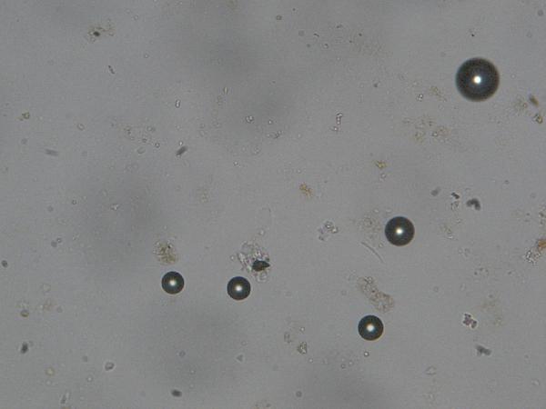
It's easy to differentiate chysophycean cysts from diatoms. Cysts are generally heavily silicifed, spherical or ovoid in shape, with a single circular pore at one end that may or may not have a collared extension. The cyst exterior is variously ornamented and can be smooth, and with or without spines, bumps, ridges, or reticulate patterns. A working group has created a standardized terminology and method for describing cyst morphotypes (see Cronberg and Sandgren 1986, Duff et al. 1995, Wilkinson et al. 2001).
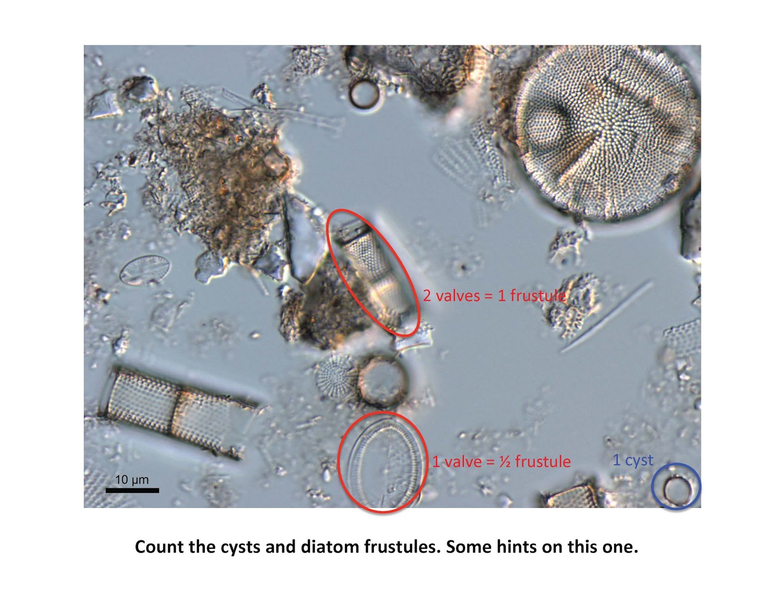
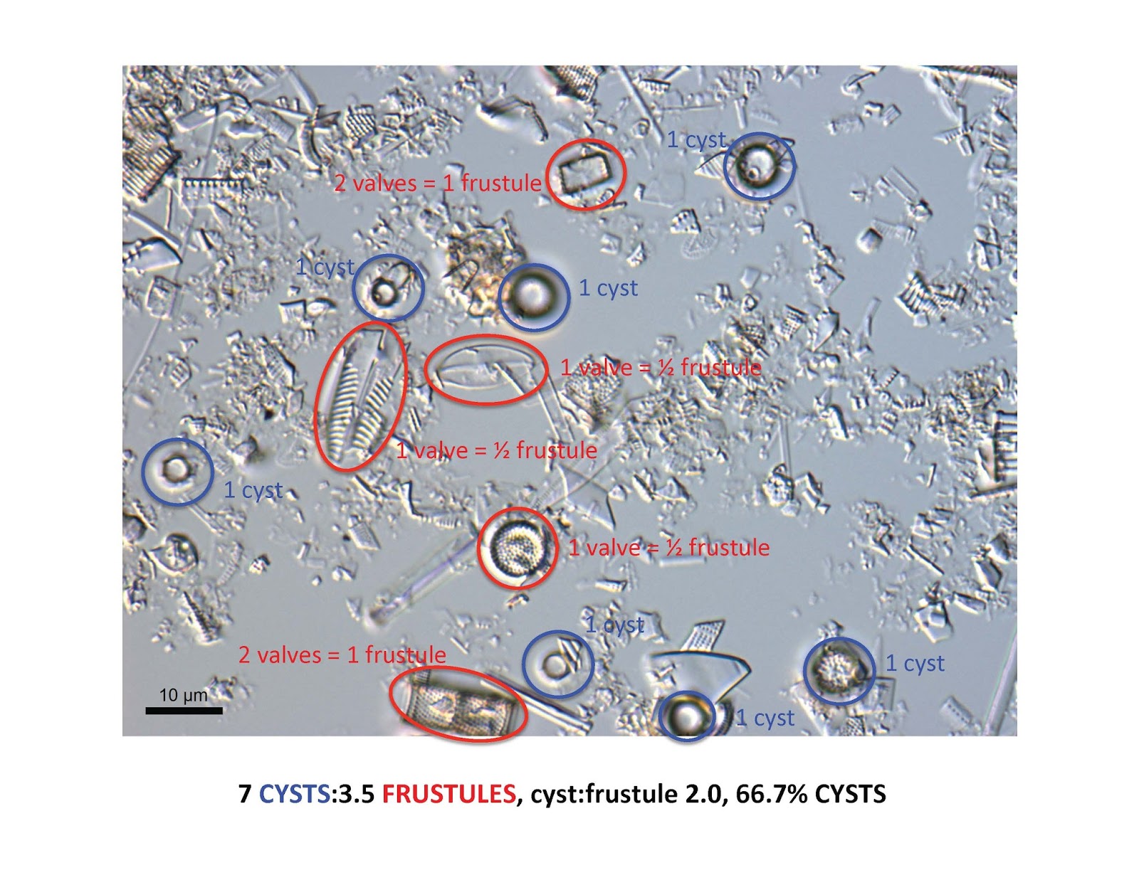
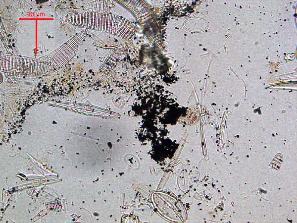
Let's look at a few images from smear slides and see how to estimate the cyst:frustule ratio in cores. Remember that diatoms have two valves in each frustule, so if you count valves you will need to divide by 2 to convert to frustules. Here's an easy one:
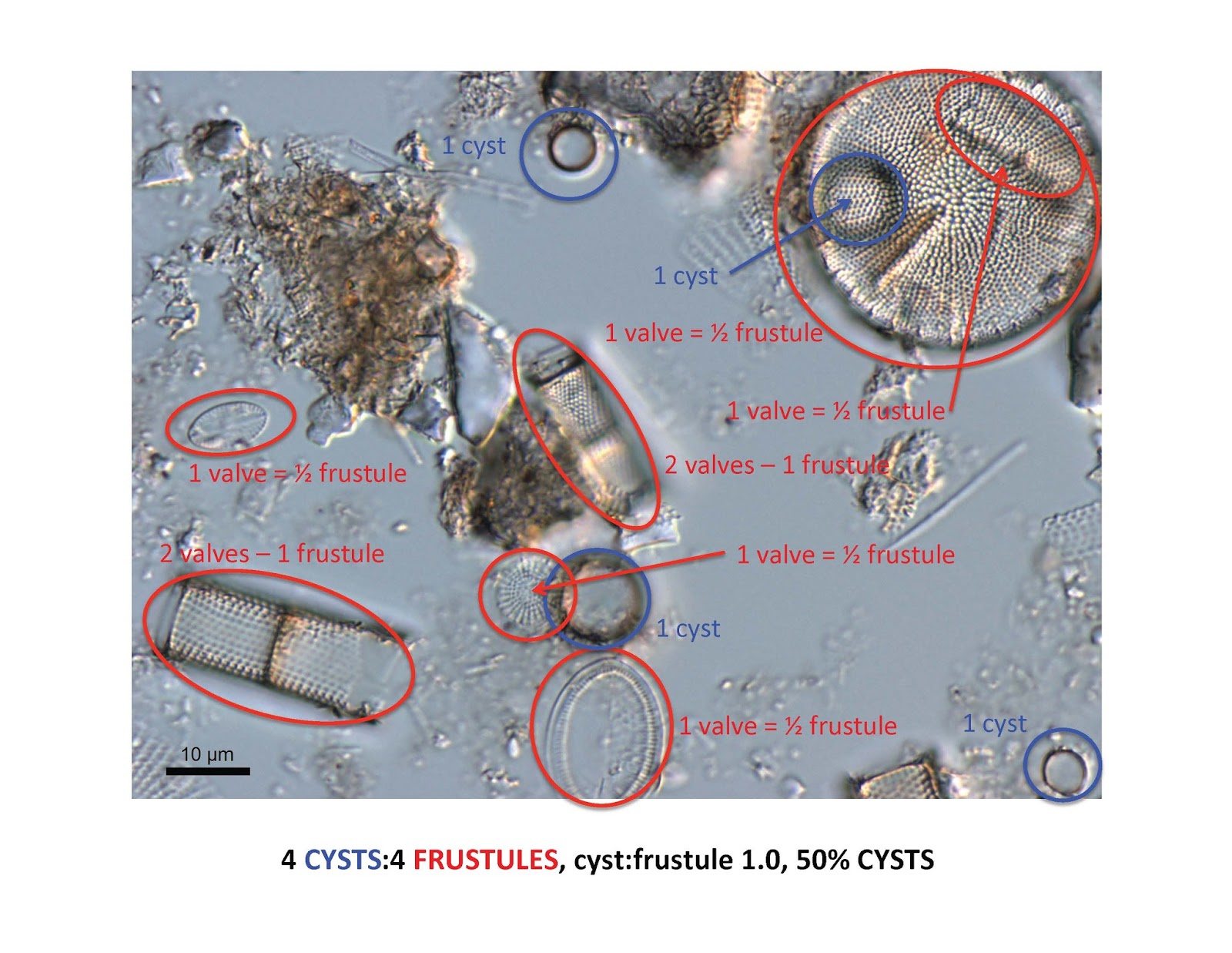
Did you find 4 cysts and 8 diatom valves making a total of 4 diatom frustules? Did you catch the cyst and diatom valve that were hiding behind the big diatom in the upper right? Remember to focus up and down to see those hidden ones. So a cyst:frustule ratio of 1:1 or 50% cysts.
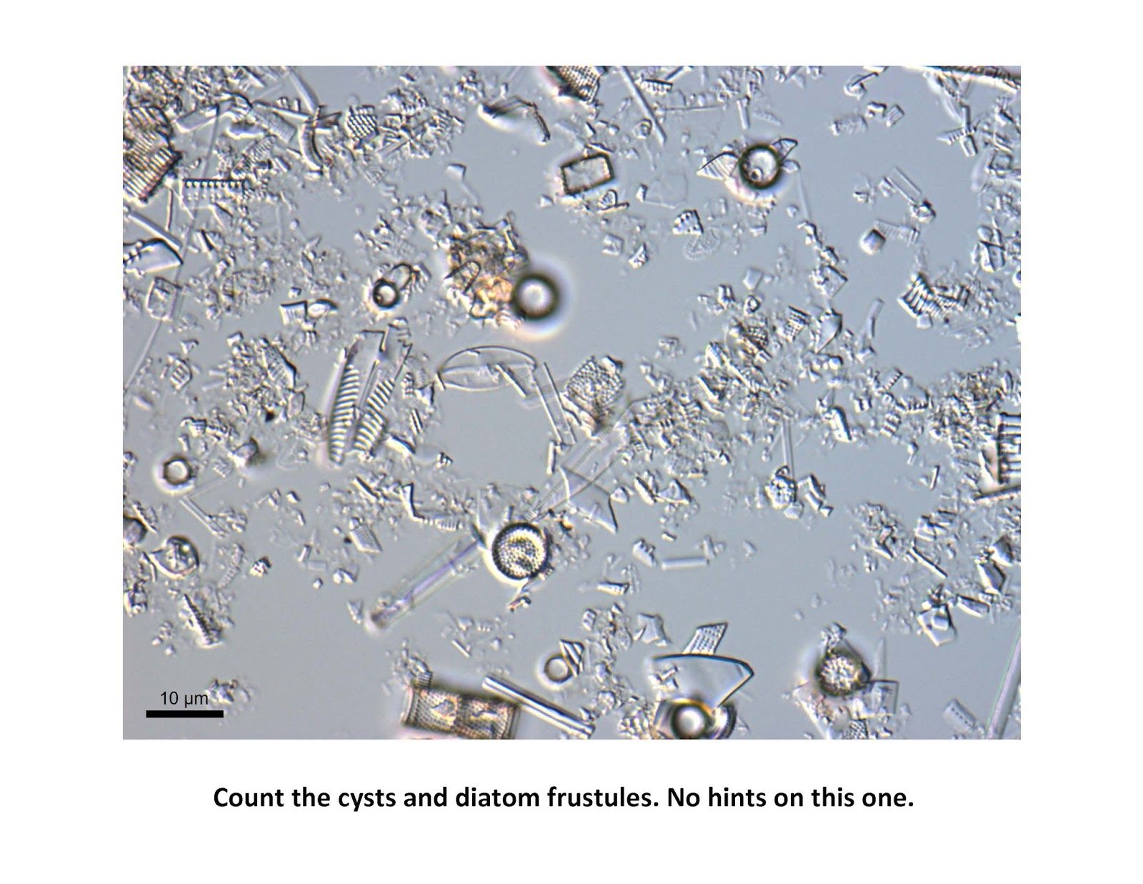
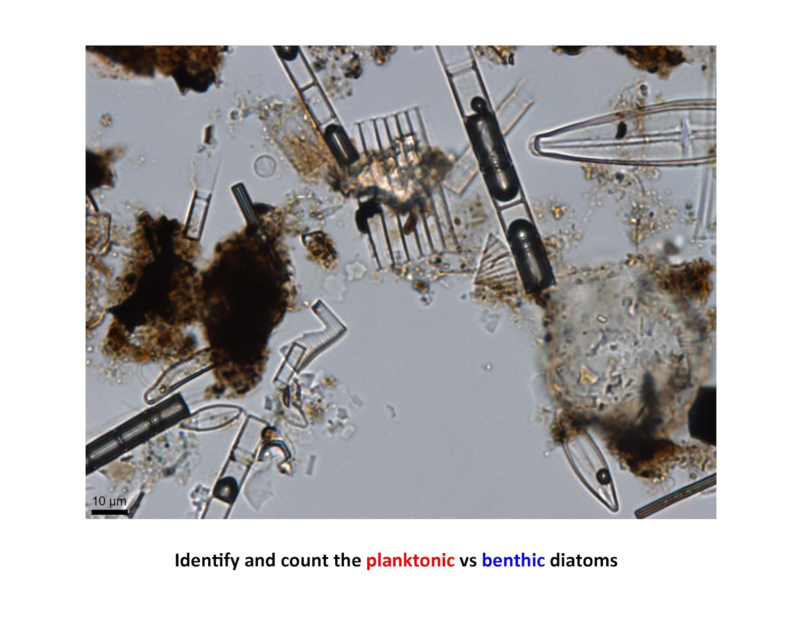
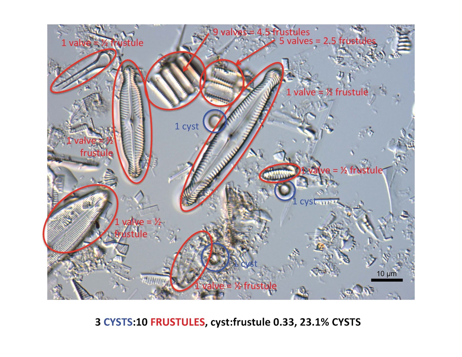
One more test of your skills, some tough diatoms on this one:
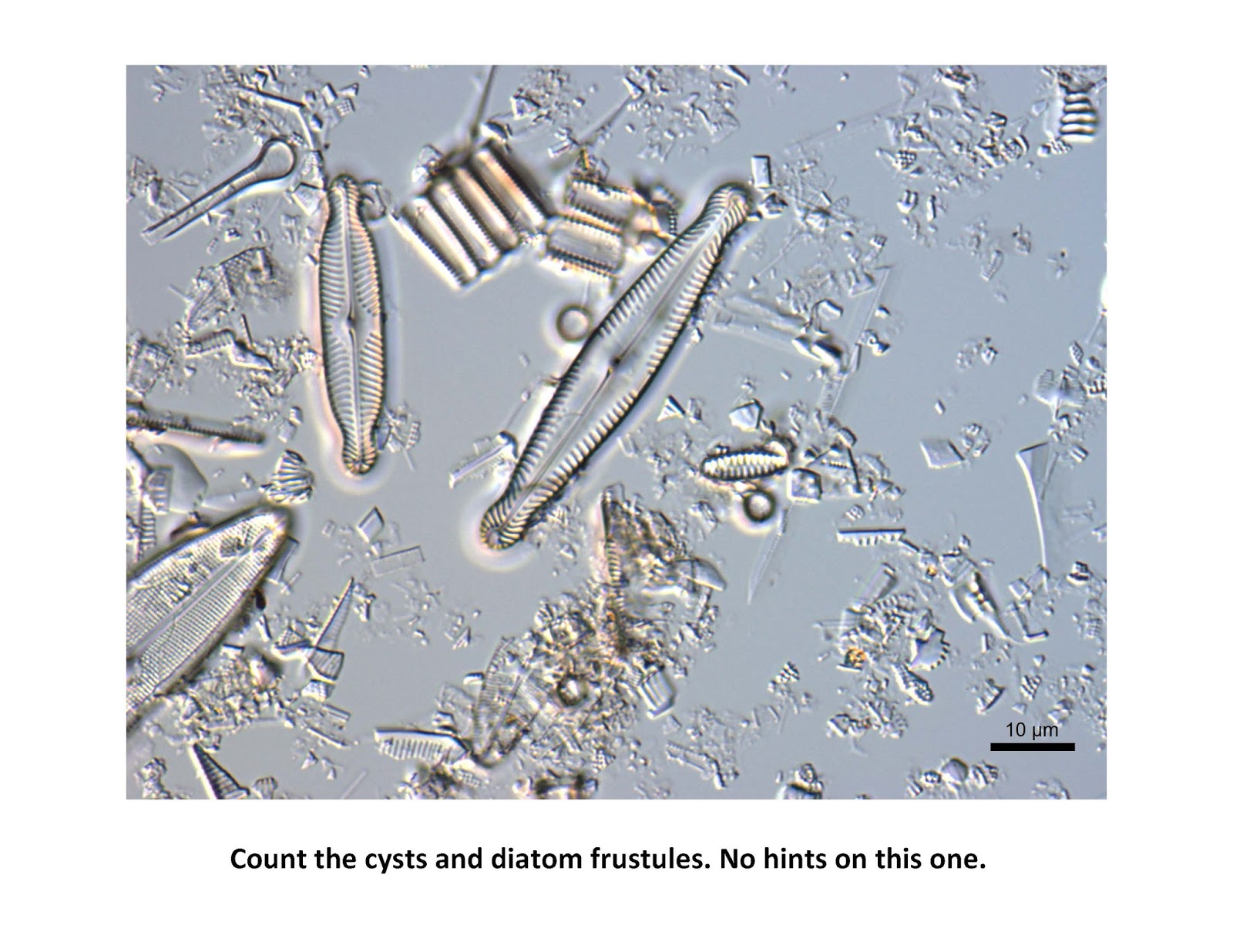
As noted above for estimating the diatom P:B ratio, it is important to count enough fields under the scope to have your estimate of cysts:frustules converge on a value for one smear slide. This may take from 400 to 600 counts, just keep a running total of the ratio as you count your random fields.
Diatom Communities –
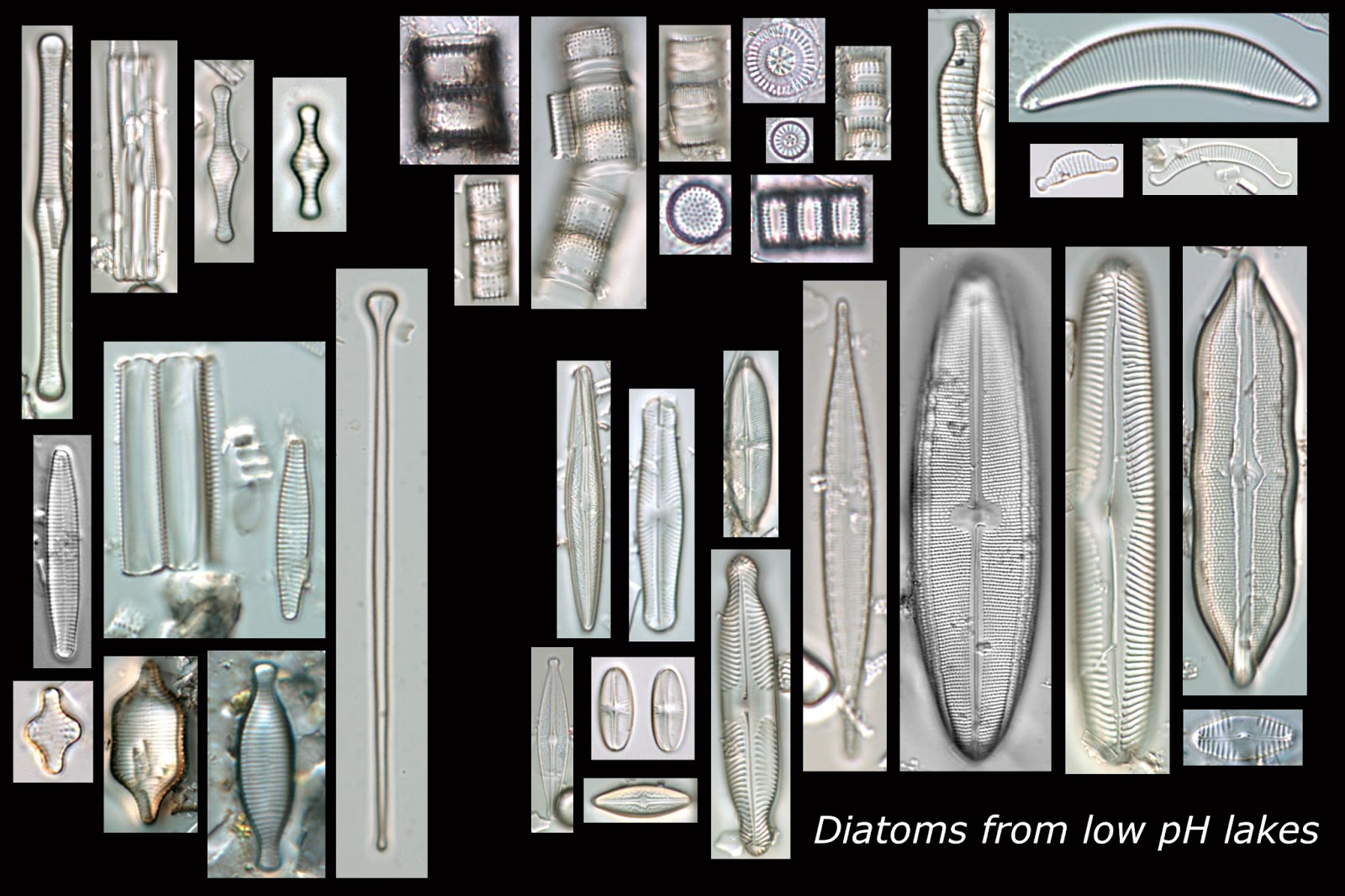
Diatom abundance and distribution are strongly controlled by a number of abiotic or environmental gradients (and biogeography-e.g., diatoms in South America are different than diatoms in North America). Among the most important gradients are pH, salinity, nutrient levels, and habitat. We earlier looked at how diatoms could be divided into their habitat preferences of planktonic vs benthic to understand lake level or nutrient changes. Here are some montages of diatoms that provide a representation of diatom communities from various lake types:
Low pH – Diatom communities from lakes with pH <7 are characterized by species that typically also prefer low conductivity and tolerate some level of DOC staining in the water. Typical acidophilic genera include Tabellaria, small-celled Aulacoseira, Asterionella and the benthic genera Eunotia, Neidium, and Brachysira.
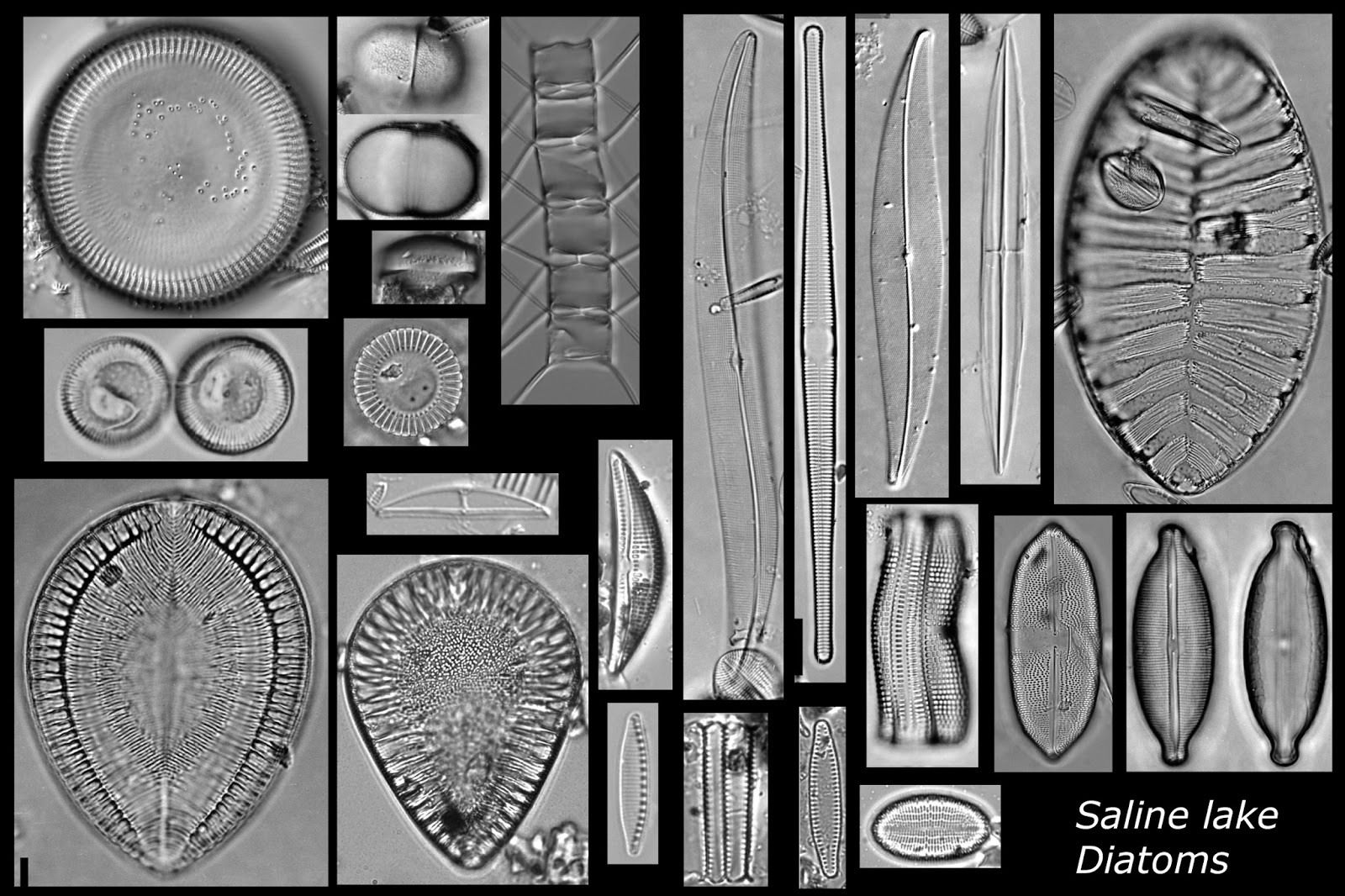
Saline lakes – Lakes are saline based on elevated concentrations of various ion combinations of notably Na+, Ca++, Mg++, SO4--, Cl-, CO3--. The transition of diatom communities from fresh water to saline is one of the most dramatic with many fresh water diatoms intolerant of high conductivity and salinity, many saline genera more represented in true marine conditions, and a set of species that are able to tolerate a wide range of salinity. These include the genera Chaetoceros and its resting spores, saline or tolerant Cyclotella, Amphora, Halamphora, Anomoeoneis, Cocconeis, Epithemia, Surirella, Campylodiscus, Ctenophora, and Rhoicosphenia.
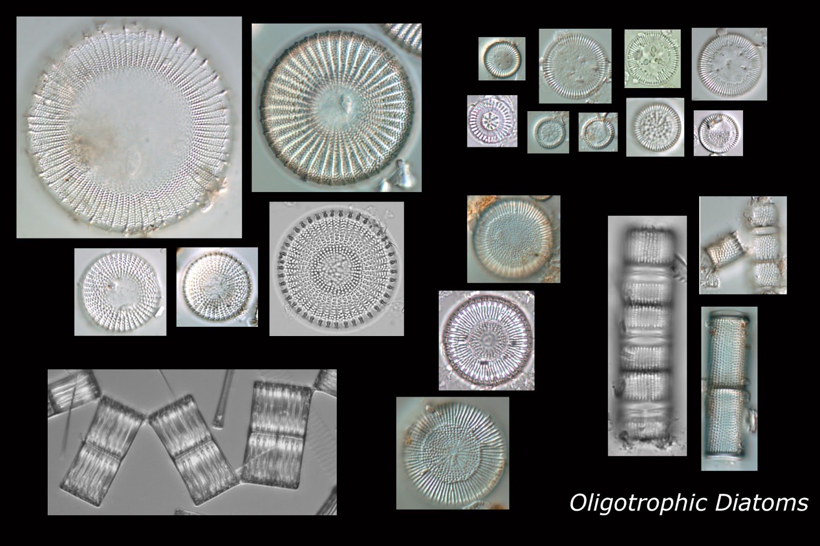
Oligotrophic or low nutrient lakes – Low nutrients, high light, deep water, and strong seasonality characterize most oligotrophic lakes. The diatoms in cores typically reflect a set of planktonic species that represent communities associated with spring and fall turnover, as well as a community that forms the "deep chlorophyll layer" and is adapted to living along the thermocline in the summer months. These species often include Cyclotella, Handmannia/Puncticulata, Stephanodiscus, Aulacoseira, Asterionella, and long-celled Tabellaria and Ulnaria species.
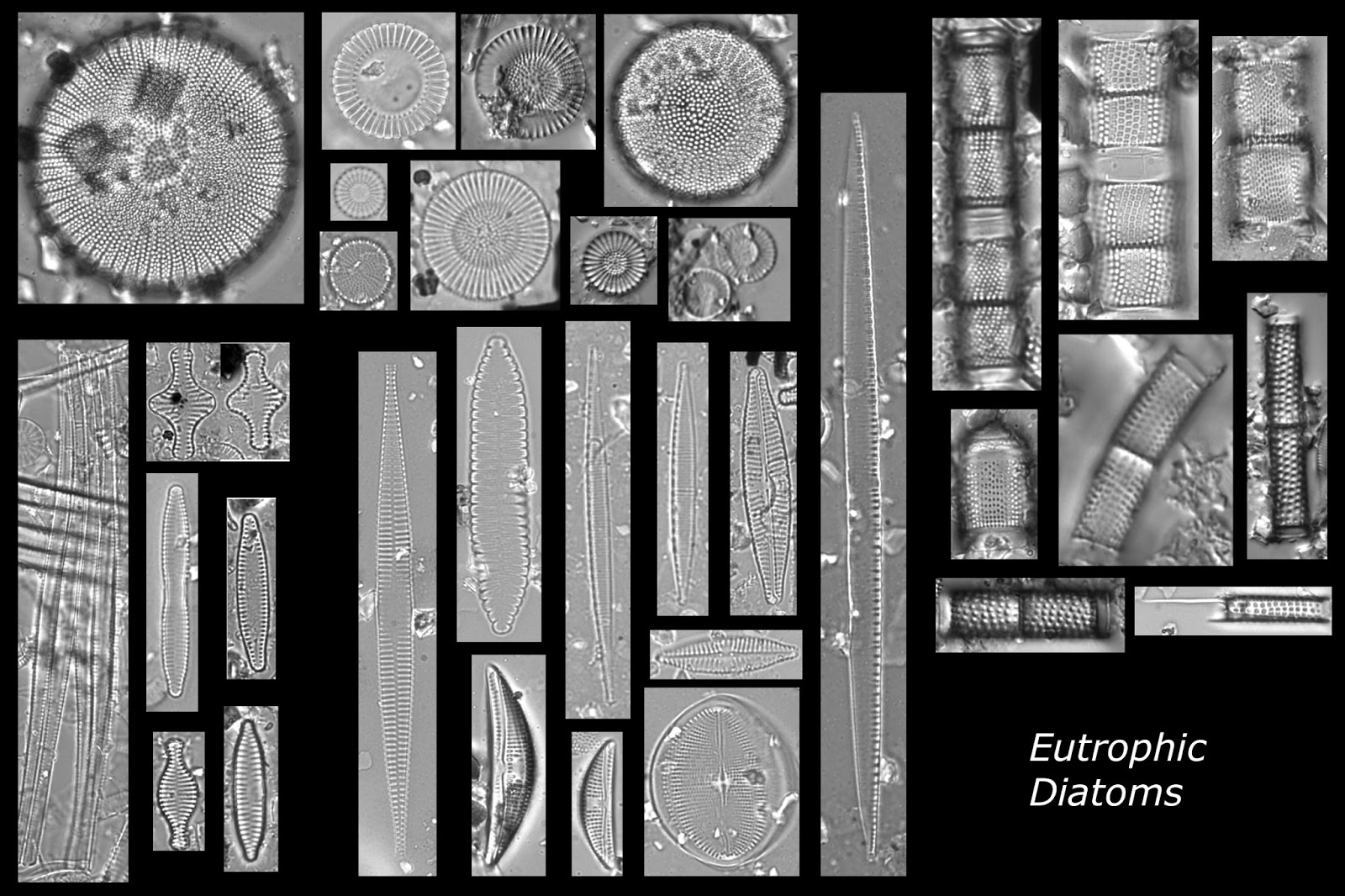
Eutrophic or high nutrient lakes – Many lakes suffer from excess nutrients and diatom communities shift in both composition and to greater abundance as nutrient levels increase. Diatom taxa that thrive under high nutrients include small Stephanodiscus, Cyclostephanos, some Aulacoseira, Fragilaria, Pseudostaurosira, and Staurosira species.
References cited:
Cronberg, G. & C. D. Sandgren. 1986. A proposal for the develop- ment of standardized nomenclature and terminology for chrys- ophycean statospores. In Kristiansen, J. & R. A. Andersen (eds), Chrysophytes: aspects and problems, Cambridge Univer- sity Press, Cambridge: 317–328.
Cumming, B. F., Wilson, S. E., & Smol, J. P. (1993). Paleolimnological potential of chrysophyte cysts and scales and of sponge spicules as indicators of lake salinity. International Journal of Salt Lake Research, 2(1), 87-92.
Duff, K. E., B. A. Zeeb & J. P. Smol, 1995. Atlas of Chrysophycean cysts. Kluwer Academic Press, Dordrecht, The Netherlands, 189 pp.
Edlund, M. B., Engstrom, D. R., Triplett, L., Lafrancois, B. M. and Leavitt, P. R. 2009. Twentieth-century eutrophication of the St. Croix River (Minnesota-Wisconsin, USA) reconstructed from the sediments of its natural impoundment. Journal of Paleolimnology 41: 641-657. DOI:10.1007/s10933-008-9296-1
Ryves, D. B., Juggins, S., Fritz, S. C., & Battarbee, R. W. (2001). Experimental diatom dissolution and the quantification of microfossil preservation in sediments. Palaeogeography, Palaeoclimatology, Palaeoecology, 172(1), 99-113
Sicko-Goad, L., Stoermer, E. F., & Kociolek, J. P. (1989). Diatom resting cell rejuvenation and formation: time course, species records and distribution. Journal of Plankton Research, 11(2), 375-389
Smol, J. P. (1985). The ratio of diatom frustules to chrysophycean statospores: a useful paleolimnological index. Hydrobiologia, 123(3), 199-208.
Smol, J. P. (1988). Chrysophycean microfossils in paleolimnological studies. Palaeogeography, Palaeoclimatology, Palaeoecology, 62(1), 287-297.
Smol, J. P. (1995). Application of chrysophytes to problems in paleoecology In: Chrysophyte algae: ecology, phylogeny and development, p. 303.
Wilkinson, A.N., Zeeb, B.A., and Smol, J.P. 2001. Atlas of chrysophycean cysts. Volume II. Dev. Hydrobiol. 157: 1–169.
Wolin, J. A., & Stone, J. R. (2010). Diatoms as indicators of water-level change in freshwater lakes. The diatoms: applications for the environmental and earth sciences, 174-185.
Zeeb, B. A., & Smol, J. P. (2001). Chrysophyte scales and cysts. In Tracking environmental change using lake sediments (pp. 203-223). Springer Netherlands.
Zeeb, B. A., & Smol, J. P. (2001). Chrysophyte scales and cysts. In Tracking environmental change using lake sediments (pp. 203-223). Springer Netherlands.
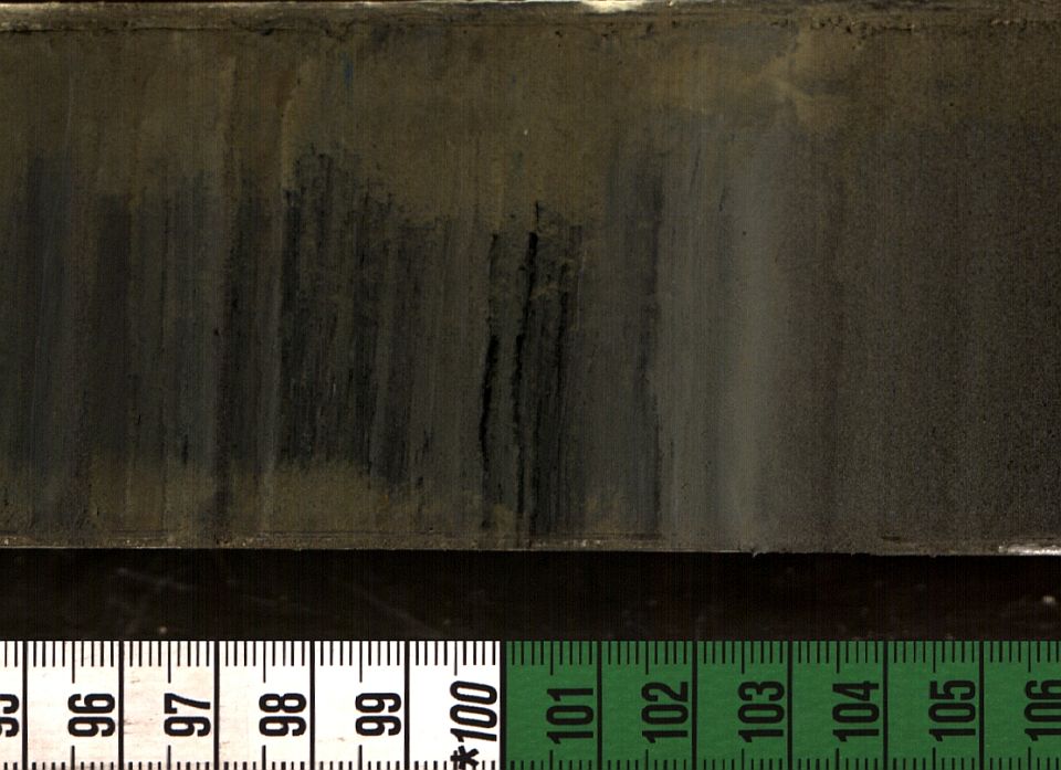
/PRES-MTN12-12B-3L-1_4x_ppl_49cm_sand.jpg)